Monday, 15 April 2013

Mapping the Gyama (Jiama) mine landslide from press images

Page Redirection

This blog has moved to a new home, if you are not redirected automatically, follow the link to stressdriven.com


Just under three weeks ago a catastrophic landslide claimed the lives of 83 workers at a copper/gold mine in China's Tibet Autonomous Region. The victims are reported to have been local workers employed by a Chinese national mining company. Many details of this tragic event are described in news reports, and summarized on Dave Petley's landslide blog, where a recent post sparked my interest. Dave makes reference to official reports that attribute the cause of the event to fracturing of natural gravel on the slope, but notes on his blog that recent Google Earth images from May and August last year show clear evidence of mountain top mining and end-tipping of waste onto a slope in the region. Dave suggests that the unusually long runout of the event may have been aided by the fractured nature of the gravels in the initiation zone, and suggests this mining activity may have had something to do with it.

A press photo of the rescue crews working at the site of this very large, highly mobile landslide. 

Although there is understandably a large amount of press coverage regarding the event, there has been very little information on the landslide itself, and most reports focus on the sometimes thousands of rescuers who have been working at the site. Images in the media do, however, show large parts of the landslide, and offer a good opportunity to illustrate how tools such as Google Earth can be used to map 3D structures from such 2D photographs. While there are a number of commercial and non-commercial software packages that currently allow users to generate 3D point clouds from multiple photographs, there are few that allow details from photographs to be projected onto digital elevation models. Some architectural software such as Sketchup allow the mapping of photographic textures onto simple geometries, but as far as I know there is nothing currently available for geotechnical applications. 

The above press photo overlaid on a Google Earth terrain model using the Add>Photo dialogue.

The Add>Photo dialogue in Google Earth is one tool which provides a simple means of combining on-site photographs with spatial geodata. This first requires that a user can reasonably accurately locate the point from which a photograph was taken. In this case, the task was not too difficult, as the existing mining roads provided me with features to "walk along" using the 'Ground level' option in GE. I could then use features in the photos to locate the most likely observer positions.  

Options in the dialogue allow full control over image positioning and transparency.

Next, using the 'Photo' tab of the 'Add Photo' dialogue, I changed the heading, tilt, roll, and field of view, to match features in a semi-transparent photo with those on the Google Earth model. By zooming out of the photo a little I could then approximately map the landslide extents 'through' the photos using the Add>Polygon tool. This step required some trial and error, as for some reason it only allowed me to move nodes in the lower left corner of the screen, however, in an hour I was able to map the region of the landslide (indicated in grey in the lower figure). Although the photographic coverage of the valley is incomplete, I could also infer a potential source region (in orange), and derive the pre-mining valley long-profile indicated in the figures below (see my previous post for info on this tool). A .kmz file containing the data for Google Earth is available for download at the bottom of this entry (I take no responsibility for it's accuracy), to view photos from the photographer positions simply click on the camera icons once the file is loaded in the Google Earth browser. 

A map of the visible landslide deposit (grey) and source area (orange) inferred from the 
run-up of landslide debris in the valley. Note the steep grey and white slope related 
to recent mining activity at the inferred source location. Cameras and text 
indicate the location of images used to 'map' the landslide.

A long-profile of the landslide source and runout zones. Note the slope gradient prior 
to the dumping of spoil was ~50% (22.5 deg). This is already approaching that of 
many natural talus slopes containing loose gravel (typically <35 deg) and clearly 
does not leave much room for storage of non-engineered mining waste on the slope.

This analysis provides some interesting insights into the event. The BBC video image looking toward the landslide source appears to show that debris ran from left to right across the valley floor, and partially into the right-hand side catchment before flowing down-valley. This suggests the source was in fact from the upper left, and may correspond to the location of what appear to be end-tipped gravels in recent mid- and late-2012) satellite images. In addition, these images show that at least late last year, there was no settlement capable of supporting 80 workers within the landslide runout zone. The majority of structures are located on the ridge crest, and close to the excavation site. While it is possible that a new camp was erected after the satellite images were taken (there seems to be some ongoing road construction), it would be very disturbing to discover that any, let alone so many, workers were operating on such a steep end-tipped gravel slope adjacent to the mining site. 

Saturday, 16 March 2013

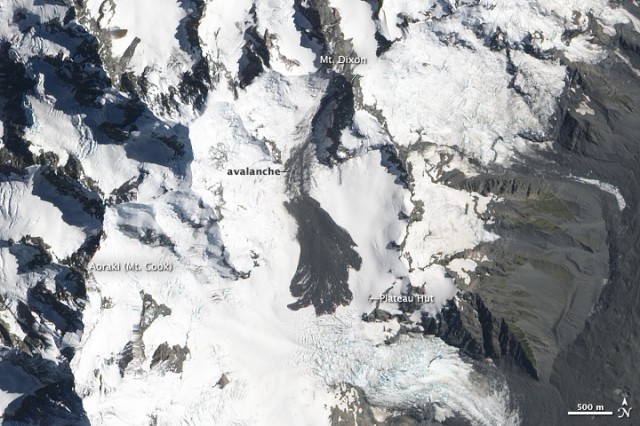
Exploring the Mt Dixon rock avalanche

Page Redirection

This blog has moved to a new home, if you are not redirected automatically, follow the link to stressdriven.com


In my last post I discussed the growing volume of geodata available online - and in particular ways in which it can be accessed by freely available GIS software. This kind of accessibility has great potential for geoscientists, and among other uses (e.g. teaching, structural geology) perhaps is a step toward 'crowdsourcing' geotechnical expertise for geohazard identification and emergency response. We can take a look at the 2013 Mt Dixon rock avalanche to see an example of this (see Dave Petley's landslide blog for a very interesting discussion on this event).


A NASA EO-1 ALI image of the Mt Dixon rock avalanche deposit (credit: The Landslide Blog)

By draping the NASA image over topography in GE, and including the geological units, fault traces, and structural measurement layers from the GNS repository we can get some understanding of the lithological and structural setting of the failure.


Satellite image overlay of the rock avalanche including structural and lithological data
Click here to download the data for Google Earth 

The light blue shading indicates the failure occurred in interbedded greywacke and argillite (perhaps no surprise there), and we might infer that structure in the region of the landslide is possibly affected by the westerly-dipping faults present on the lower valley wall. The orange markers indicate the location of structural measurements, and support a regional dip azimuth of between 260 and 330 deg, with an inclination of between 60 and 80 deg. This is a similar orientation to the planar rock slope immediately south-east of Mt Dixon, and would indicate the initial movement direction was perpendicular to the local bedding orientation. Using the "Add path" tool in GE, we can draw a long profile to investigate the pre-failure topography of the runout zone. If we select the new path in the menu, the "Show elevation profile" tool will produce a plot of elevation vs. distance along the path.


Mt Dixon rock avalanche runout path, indicating an elevation loss of ~890 m, and reach angle of 29% (16 deg). The red arrow on the map indicates the transition to deposition, and is reflected by the vertical grey marker on the elevation profile. This appears to be the base of a crevasse field marking a steepened section of the glacier surface.


While these observations are relatively simple, I hope they provide some inspiration to realize the potential for what is a growing volume of readily-accessible geodata, particularly when it can be incorporated in a free 3D mapping platform such as Google Earth.

Wednesday, 13 March 2013

Visualizing geodata in 3D

Page Redirection

This blog has moved to a new home, if you are not redirected automatically, follow the link to stressdriven.com


After spending some time working on the Bavaria maps pages (both the Earth and Maps pages work now!), I recently went in search of a way to project the same data in a vector format. At the moment I use the GDAL library (specifically gdalwarp and gdal2tiles) to convert georeferenced .tiff files to a .png format for projection in Google Earth (GE). These are raster files, just the same as the .jpg's that come from your digital camera, and each pixel is assigned a different colour. Using the data in this way has some issues, however, as the resolution of the images is limited, there's no way to attach metadata, and serving up all the image files puts a reasonable load on the server.... In contrast, vector formats allow us to define a shape by coordinates, then tell the computer a texture or colour to fill the shape, and  present the same data with essentially has no resolution limits (though it of course depends on the accuracy of the data collection). In addition vector files can contain metadata with links to external webpages, and are usually about 10% the size of the raster images. 

After passing through OneGeology.org, I landed at the GNS GeoServer website. OneGeology is one of those 'logical' collaborative efforts much like Wikipedia or OpenStreetmap for geological maps... for some time now, Geological data has been provided online using the .wms format as a means of connecting remotely served geological data to whatever GIS software you're running on your PC (see here for an example). It's really a great step forward, I think you could say that this initiative now provides geological data of the whole world at some resolution for free. It is, however, still a bit slow and somewhat disorganized at the moment, at least on the OneGeology portal... But as it's a true cutting-edge combination of science and IT, I think the fact that it's there is really fantastic.

The OneGeology portal links .wms data from various servers around the world, one of which is located at GNS in New Zealand. While I'm new to this, the GNS site is one of the best geodata services I've come across. The portal (once you click on Data>layer preview) provides access to 1:1M and 1:250k geodata for the whole country in a wide range of formats... including .kml for GE. This can be accessed as network links streamed off the server (for GE, first download the .kmz file by clicking here), or (for example) as a .kml file to download to your computer (this is a bit faster, check the portal). 

Google Earth screenshot showing vector-based geology of the Mt Cook region 
(data credit: GNS & Google)

I'm told by the guys and girls at GNS that the data-serving side is a true 'work in progress' (a client upgrade will happen next week), and I think the future looks exciting for the users throughout the geoscience world.

Sunday, 3 March 2013

It's time to do this!

Page Redirection

This blog has moved to a new home, if you are not redirected automatically, follow the link to stressdriven.com


Hi all,

Over the last few years I've spent a lot of time working in the Alps - learning about the valley geomorphology, slope instabilities, bedrock properties... enjoying the steep valleys, long trails, alternately hot and freezing weather, and supermarkets closed at lunchtime. 

Looking north from the Zugspitze - Feb 2013
A German version of steep valleys and freezing weather;
A view from the top of the inaccessible (for this scientist) north wall of the Zugspitze this Feb.

At the same time I've become reliant on web-based GIS as a means of maintaining field data, using tools such as Google Earth to keep it accessible even when I wasn't in the office - or when the office was not as ordered as it should have been. As I begun to generate modelling data, the simple format, and flexibility of .kml (the .xml?-based language of GE) lent itself to quickly producing results out of a number of softwares... 

The ability to compare field data to model results in a 3-D GIS environment, and share and discuss results with colleagues around the world without requiring any special software, provided some of the greatest insights during my time in Zurich.

I now have a reasonably large library of code, tools, and .kml-based geo data that grew with the project, but never really reached a 'mature' stage... Over the next months I hope to begin outlining some of the methods and tools I found most useful... and while I'm not an html-monkey I'll try to present some of the ideas, concepts, useful websites, and codes using the awesome google .api library.

To start, I've linked the 1:500 000 geological maps of Switzerland, (Liechtenstein), and Germany as Google Earth and Google Maps overlays on my "Online maps" page. In the next days I'll describe where to find the data, how to adapt it, and some of the benefits of having something like this available in a 3-D open source platform!


3D Geology of the Swiss alps looking out over Thun, Tichino, and south toward Italy